Creating a visual CV
... a nice addition to a text-based CV
By Andrea Rau in Tips and tricks
October 31, 2018
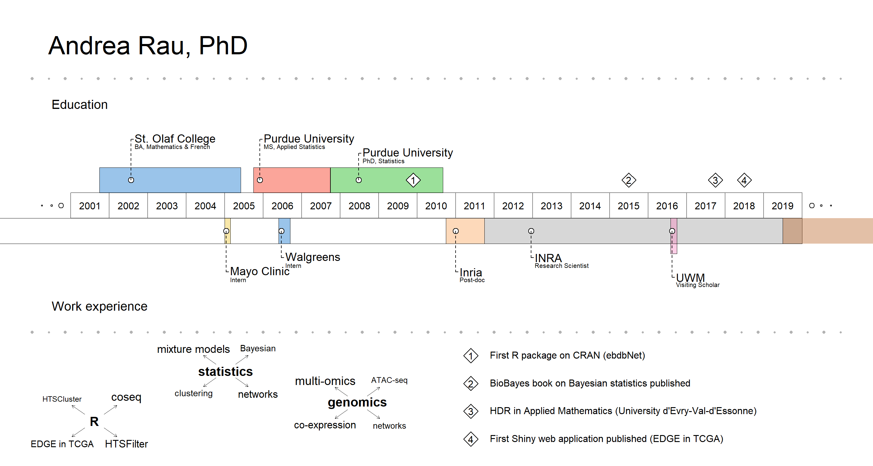
This is a short post to provide details on how I created the visual CV that is included on my homepage. I got the idea for doing this from a tweet from the awesome Mara Averick about an R package called VisualResume by Nathaniel Phillips:
Once VisualResume is installed from GitHub (via devtools) and loaded, I just modified the Walter White example, resized the plot directly in the RStudio plot window, and exported to PNG.
library(VisualResume)
VisualResume::VisualResume(
  titles.left = c("","Andrea Rau, PhD",  ""),
  titles.right = c("", "", ""),
  titles.left.cex = c(1,  4, 1),
  timeline.labels = c("Education", "Work experience"),
  timeline = data.frame(title = c("St. Olaf College", "Purdue University",
                                  "Purdue University", "Inria", "INRA", "UWM", "UWM",
                                  "Mayo Clinic", "Walgreens"),
                        sub = c("BA, Mathematics & French", "MS, Applied Statistics",
                                "PhD, Statistics", "Post-doc",
                                "Research Scientist", "Visiting Scholar",
                                "AgreenSkills+ Fellow", "Intern", "Intern"),
                        start = c(2001.75, 2005.75, 2007.75, 2010.75, 2011.75,
                                  2016.58, 2018783, 2005, 2006.4),
                        end = c(2005.42, 2007.74, 2010.67, 2011.75, 2020, 2016.75,
                                2019.5, 2005.15, 2006.7),
                        side = c(1, 1, 1, 0, 0, 0, 0, 0, 0)),
  milestones = data.frame(title = c("BA", "MS", "PhD"),
                          sub = c("Math/\nFrench", "Applied\nStatistics",
                                  "Statistics"),
                          year = c(0, 0, 0)),
  events = data.frame(year = c(2009.9, 2015.5, 2017.75, 2018.5),
                      title = c("First R package on CRAN (ebdbNet)",
                                "BioBayes book on Bayesian statistics published",
                                "HDR in Applied Mathematics (University d'Evry-Val-d'Essonne)",
                                "First Shiny web application published (EDGE in TCGA)")),
  interests = list("R" = c(rep("coseq", 4), "HTSCluster",
                           rep("HTSFilter", 3), rep("EDGE in TCGA", 2)),
                   "statistics" = c(rep("mixture models", 6),
                                    rep("clustering", 3), rep("networks", 5),
                                    rep("Bayesian", 3)),
                   "genomics" = c(rep("multi-omics", 8), rep("ATAC-seq", 2),
                                  rep("co-expression", 6), rep("networks", 3))),
  year.steps = 1
)